Machine Learning (ML) in Bioinformatics

Decision Trees

What are decision trees?

A decision tree is a tree structure that resembles a flowchart where an internal node represents a feature, the branches represent decision rules, and each leaf node defines the outcome.

Vocabulary

...

The root node is the top node in a tree, and it learns to partition based on the attribute value and partitions the tree in a recursive manner called recursive partitioning.

Decision trees are widely used because they are simple to understand and interpret and can handle high-dimensional spaces and large numbers of training examples. However, they do have some limitations, such as being prone to overfitting and performing poorly on very noisy data.

To build a decision tree, we start at the root node and split the data on the feature that results in the purest child nodes (i.e., the child nodes contain samples that are as similar as possible).

We then repeat this process for each child node, splitting the data on the feature that results in the purest child nodes until the leaf nodes contain pure samples (i.e., all the samples in the leaf node belong to the same class).

Here is an example of a simple decision tree that predicts whether or not an individual will play foobal based on the weather conditions:

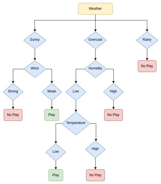
In this example, the root node is "Weather," and the leaf nodes are "No" and "Yes." The branch nodes are "Sunny," "Overcast," and "Rainy."

The decision tree predicts by starting at the root node and working its way down the tree based on the values of the features. For example, if the outlook is overcast, the decision leads to the next decision node, the "Wind."

If the wind is weak, the tree would predict that the individual will play football (Play). If the outlook is "Overcast," the next decision node is "Humidity." If the humidity is "High," the tree would predict that the individual will not play football (No play).

If the "Humidity" is "Low," the tree leads to the next decision node, "Temperature." If the temperature is "Low," the tree predicts that the individual will play, as opposed to if the temperature is "high," the tree would predict that the individual will not play football (No play).

Building decision trees

Several algorithms can be used to build decision trees, including:

ID3
(Iterative Dichotomiser 3):

ID3 is one of the most popular decision tree algorithms. It uses entropy and information gain to construct a decision tree.

C4.5 (Classification and Regression Tree):

C4.5 is an extension of ID3. It can handle both continuous and categorical data and uses an information gain ratio instead of entropy.

C5.0:

C5.0 is an improvement over C4.5 and is more resistant to overfitting.

CART (Classification and Regression Tree):

CART is a decision tree algorithm that can handle both continuous and categorical data. It creates binary trees and uses the Gini index as the splitting criteria.

CHAID (Chi-squared Automatic Interaction Detection):

CHAID is a decision tree algorithm that can handle both continuous and categorical data. It uses the chi-square test to find the best split.

We can build a decision tree by following these steps:

1. Select the best feature. Use Attribute Selection Measures (ASM). It is a method used in data mining for data reduction and record splitting.
2. Place the best attribute as a decision node and break the dataset into subsets.
3. Start building the tree by repeating the above process recursively for each child and stop when one of the following conditions matches:
• All the tuples belong to the same attribute (feature) value.
• There are no more attributes.
• There are no more instances.

There are several attribute selection measure techniques that we can use to select the best attribute:

Gini index:

It measures the impurity of the input set.

Entropy:

It calculates the impurity of the input set.

Misclassification error:

It calculates the misclassification error rate.

Gain Ratio:

It calculates the relative reduction in entropy.

Chi-square:

It calculates the statistical significance of the differences between sub-nodes and parent node.

Pruning decision trees

Pruning is a technique used to improve the generalization of a decision tree by reducing the size of the tree. It does this by removing nodes that do not significantly improve the prediction accuracy of the tree.

There are two types of pruning techniques:

1. Pre-pruning

Pre-pruning involves setting the minimum number of samples required to split an internal node or the maximum depth of the tree. The minimum number of samples prevents the tree from growing too deep and overfitting the training data.

2. Post-pruning

Post-pruning involves building the decision tree and removing nodes that do not significantly improve prediction accuracy.

To perform post-pruning, we follow the following steps:

1. Split the training data into training and validation sets.
2. Build a decision tree using the training set.
3. Evaluate the performance of the tree on the validation set.
4. Identify the nodes that do not provide a significant improvement in the prediction accuracy and remove them.
5. Repeat steps 3 and 4 until the performance of the tree on the validation set stops improving.

There are several approaches to post-pruning:

Reduced error pruning:

This method removes a node if the accuracy of the tree decreases by less than a threshold after the node is removed.

Minimum error pruning:

This method removes a node if the accuracy of the tree increases after the node is removed.

Minimum complexity pruning:

This method removes the nodes that result in the smallest increase in the complexity of the tree.

Minimum description length pruning:

This method removes the nodes resulting in the tree's shortest description.

Decision tree ensembles

Decision tree ensembles are machine learning models that consist of multiple decision trees and are used to improve the performance and predictive power of a single decision tree.

Random forests and gradient boosting are two of the most popular types of decision tree ensembles. Random forests are an ensemble model that combines the predictions of multiple decision trees trained on different subsets of the training data.

The idea behind random forests is that each decision tree will make predictions that are slightly different from the others. By averaging the predictions of all the trees, we can get a more accurate and stable prediction.

To build a random forest, we follow the following steps:

1. Select N random samples from the training data with replacement.
2. Build a decision tree for each sample.
3. For each tree, select M random features without replacement.
4. Train the tree using the selected features.
Make predictions using all N trees and return the majority vote (for classification) or the average (for regression).

Gradient boosting is another ensemble model that combines the predictions of multiple decision trees differently. In gradient boosting, the trees are trained sequentially, with each tree trying to correct the mistakes of the previous tree.

To build a gradient-boosting model, we follow the following steps:

1. Initialize the model with a constant value (for regression) or the class probabilities (for classification).
2. For each tree, fit a decision tree to the residual errors of the previous tree.
3. Make predictions using all the trees and return the sum of the predictions.

Random forests and gradient boosting are powerful machine learning algorithms that have been used to achieve state-of-the-art results on various tasks. They are widely used in the industry and have proven effective in various applications, including image classification, natural language processing, and predictive modeling.

Evaluating the performance of decision trees

Evaluating the performance of a decision tree is an essential step in the model-building process, as it helps us understand how well the model can make predictions on unseen data.

Several metrics can be used to evaluate the performance of a decision tree, including accuracy, precision, recall, and F1 score.

Accuracy is the proportion of correct predictions made by the model, and it is the total count of correct predictions divided by the total count of predictions.

Precision is the proportion of correct positive predictions made by the model. It is the count of true positives divided by the total count of both the true positives and false positives.

The recall is the proportion of positive instances that the model correctly predicted. We can calculate the recall by dividing the total count of true positives by the sum of the true positives and false negatives. The F1 score is the harmonic mean of precision and recall, where the best score is 1.0, and the worst is 0.0.

In addition to these metrics, it is also essential to evaluate the performance of a decision tree using cross-validation.

Cross-validation is a technique that involves dividing the training data into folds, training the model on one fold, and evaluating it on the other fold. We repeat this until all folds have been used for evaluation. After, we average the model's performance across all the folds.

References and further reading